Blog
Why is inequality in South Africa higher than in Germany?

The understanding of inequality requires the analysis of changes in income distributions across countries and over time as well as the identification of its drivers. To achieve this we use different statistical tools to identify the distributional patterns and summarize the results using inequality indices. The use of decomposition analysis has been particularly popular in the field for the purpose of identifying strong statistical associations, even if the identification of causality is complex in this context. There are at least three different types of common inequality decompositions: by population groups, by income sources, and regression-based decompositions.

In this article, I will use a practical case and combine these different approaches that are usually investigated independently, based on the methods proposed in Gradín (2018, 2019), where they are explained in more detail. I will use data from the Luxembourg Income Study (LIS). Inequality will be measured for disposable income per equivalent adult.¹ I will focus on two indices that have the right properties, the Mean Log Deviation (MLD) and the Gini index.² I will compare inequality in one highly unequal country (South Africa, 2012) and in one low-inequality country (Germany, 2013).

Indeed, South Africa is the country with the highest level of income inequality in LIS, while Germany has one of the lowest levels among the largest economies. Inequality in South Africa is higher than in Germany as shown in Figure 1, with the gap being 0.316 (Gini) and 0.560 (MLD).

The aim is to shed some light on the role in driving the cross-country gap in income inequality played by i) a head’s attained education,³ probably the most relevant socioeconomic characteristic, and ii) two incomes sources (net of direct taxes): ‘market income’, broadly defined here as incomes derived mainly from labor, old-age pensions and capital, and ‘public social benefits’ (other than pensions).

Figure 1 - Inequality in South Africa and Germany

Inequality decomposition by population groups

The first decomposition type implies breaking the population of each country into groups based on one socioeconomic characteristic, such as race, region, education, etc. The most common approach implies decomposing total inequality into the contribution of inequalities between groups and within groups so as to identify how strongly inequality is associated with each particular characteristic (higher share explained by the between-group component), using an index such as the Mean Log Deviation, in which the overall level of inequality is equivalent to the sum of these two components.

Inequality between groups is obtained as the level of inequality that remains after equalizing the incomes within groups in each country (assigning everyone the mean of their group). Inequality within groups is the level of inequality remaining after re-scaling individual incomes so that all groups have the same mean income in each country, which is equivalent to the sum of group inequalities, with each group weighted by its population size.⁴

It is when following the decomposition according to population groups that we know that inequality among all citizens of the world is mainly determined by differences in the average income of the country in which we live (inequality between countries), even if the within-country component is becoming more relevant over time. We also know that the urban-rural gap played an important role in the increase of inequality in China after the economic reforms, or that race, caste or ethnicity are fundamental to understand inequality in many countries, with South Africa and India standing out in this respect.

In my example, MLD bar in Figure 2, it turns out that the inequality gap between South Africa and Germany, measured by the MLD, is in part due to the striking mean income differences among educational groups in South Africa. On average the most educated group receives 15 times the income of the least educated, compared with 2.4 times in Germany. Despite being large, these between-group inequalities still explain only 39 per cent of the total gap. The main component, about 61 per cent, is due to cross-country differences in within-group inequality. That is, differences that occur among people with the same head’s educational level (regardless what their group mean income is). In South Africa your level of education determines to a larger extent where you are in the income distribution (35 per cent of inequality is between educational groups, compared to 18 per cent in Germany), there is also an even larger variability within each educational group.

Inequality decomposition by income sources

A second decomposition type is the decomposition of total inequality into the contribution of income sources (e.g. earnings, social benefits, taxes …). In its simplest and most popular version, the contribution of an income source can be measured as the change in inequality after adding that source to the other incomes (Musgrave and Thin 1948, and subsequent literature).⁵ 

Defined in this way, a source can be progressive or regressive depending on whether it contributes to making inequality lower or higher. The analysis of income sources has allowed to find out that income inequality in most countries is mainly generated in the labor market, while it is partially offset by the effect of taxes and social benefits, but with great variability across countries based on factors such as their economic structure, inequalities in human and physical capital, labor market institutions, exposition to trade or technological change, and how redistributive the tax-benefit system is, among other things.

Therefore, the second question addressed in my example, is whether the observed country gap is the result of a more disequalizing market or of a weaker welfare state in South Africa compared with Germany. For that, I compare inequality, measured by the Gini index, before and after adding public social benefits to market incomes. Inequality decreases by a similar amount in both countries: from 0.341 to 0.291 (-0.050) in Germany, and from 0.644 to 0.599 in South Africa (-0.045). The initial gap of 0.304 Gini points only slightly increases to 0.308 (Gini bar in Figure 2). It turns out that the much higher original level of market income inequality, not the smaller reduction resulting from social benefits, is the reason why inequality is higher in South Africa.

Figure 2 - Decomposing the inequality gap between South Africa and Germany by income source (Gini) and population groups (MLD)

Inequality decomposition into composition and distribution effects

Finally, the regression-based decomposition approach allows us to decompose the differential in inequality between two distributions into a composition effect (difference driven by the divergent distribution of characteristics) and an income structure or distribution effect (difference driven by how population groups are differently distributed across incomes).

For example, it is possible that a household with a given educational level obtains the same relative income in both countries and inequality is higher in South Africa simply because there are more people with lower education (and therefore lower relative earnings). In that scenario, we could say that the inequality gap is driven by a composition effect (by educational groups). Alternatively, the two countries might have the same share of the population by educational level but differ in the income distribution of each educational group.

In this case, the distribution effect would be the reason for the inequality gap that indicates to what extent educational groups are associated with more inequality in one country, i.e. some groups tend to be at the bottom and/or top of the distribution.⁶ This should not be confused with the within-group inequality discussed above because groups may differ in income variability but also in their average income.

I obtain the composition effect estimating how much of the inequality gap disappears after equalizing the distribution of educational groups in both countries (they have the same proportion of people in households with higher education, for example). I do this by constructing a counterfactual (hypothetical) distribution in which I give households in Germany the educational distribution in South Africa and repeat the exercise swapping countries (by reweighting the corresponding samples). The composition effect is the average level of inequality that has been reduced in both cases. The distribution effect indicates the inequality gap that remains when both countries are compared in terms of the population shares by educational levels.

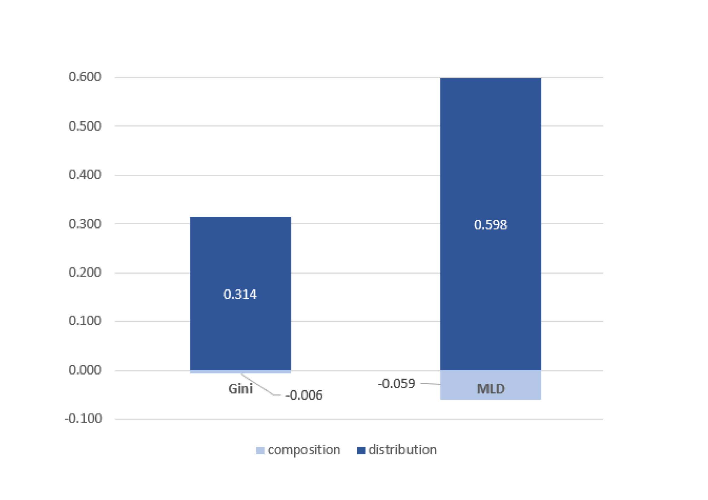
There is no doubt that the educational structure of the population in both countries is quite different, with more South Africans living in households where the head has not achieved lower secondary education (35 per cent of the population, compared to only 2 per cent in Germany) and fewer in which the head has a bachelor degree or higher education (5 per cent versus 26 per cent). Despite these striking differences, once they are removed, the inequality gap would still be similar or even higher (by 0.006 with Gini, 0.059 with MLD) as shown by the composition effects in Figure 3. Therefore, the inequality gap between the two countries cannot be described as the result of a composition effect. The entire cross-country inequality gap stems from a distribution effect, that is, from the stronger association of a head’s education level with the position of households along the income scale in South Africa.

Figure 3 - Decomposing the inequality gap between South Africa and Germany into composition and distribution effects

Combining different approaches

It is interesting to note that despite the strong connection and potential complementarities in the study of inequality among these three decomposition approaches, they have been investigated and used almost independently from each other. So far, I have shown three basic results: the inequality gap is i) mainly driven by inequality within educational groups (although between-group inequalities are also notable), ii) is generated before public social benefits are accounted for, and iii) is generated by the different income distribution of educational groups, not by their population shares being different in both countries.

My main point here is that these narratives can be connected (see Table 1). For example, if it is the income distribution of educational groups, not their size, that matters. These differences can arise because either these groups have different average incomes (between-group inequality) or different intragroup variability (within-group inequality). That is, we can reassess the role of between-group and within-group inequalities in a scenario in which both countries have the same relative group sizes, to find out that these proportions are 43 and 57 per cent (Figure 2). Thus, removing the composition effect does not significantly alter the fact that it is within-group variability that explains higher inequality in South Africa.

Similarly, one can ask whether the different income distribution of educational groups, when both countries are compared with the same educational distribution, is produced by market income or by social transfers, and then find out that after removing the composition effect it turns out that the weaker social transfers in South Africa are more relevant than suggested above in explaining the inequality gap (0.046 Gini points) but that this was partially hidden by the associated composition effect (the disproportionally larger share of South Africans with low education who benefit more from these transfers) (Figure 3). One therefore definitely needs to analyze why the labour market in South Africa generates so much inequality to understand higher inequality in South Africa (see for example, Murray et al., 2020).⁷

One can see that the largest contribution to the inequality gap is associated with households with the lowest educational level but that this is mainly the result of a composition effect (this group is disproportionally larger in South Africa). When it comes to the distribution effect, however, it is the distinct income distribution of the upper-secondary group in both countries that contributes most to the gap through market income inequality and within-group inequality.

In addition, Table 1 provides more details on the educational groups through which these effects are channeled because it is possible to identify the contribution of each group to overall inequality, or to any of its components (inequality by income source, between-group and within-group inequality, composition and distribution effects, or combinations of them).

Table 1 - Detailed decomposition of the cross-country gap

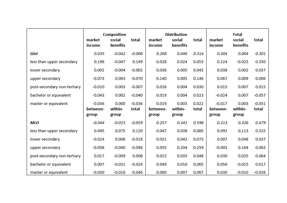
Note: Detailed composition effects include the impact of non-linearity in the relationship between group’s contribution on inequality and population shares.

References

Firpo, S.; Fortin, N.M.; Lemieux, T. (2009). “Unconditional quantile regressions”. Econometrica, 77, 953–973.

Gradín, C. (2018). “Quantifying the contribution of a subpopulation to inequality: An application to Mozambique”. WIDER Working Paper 60/2018. Journal of Economic Inequality (forthcoming).

Gradín, C. (2019). “Inequality by population groups and income sources: Accounting for inequality changes in Spain during the recession”. WIDER Working Paper 73/2019.

Leibbrandt, M.; Green, P.; Ranchhod, V. (2020). “South Africa: The top-end, labour markets, fiscal redistribution and the persistence of very high inequality”. In C. Gradín, M. Leibbrandt, and F. Tarp (eds.) Inequality in the development world. Oxford University Press, forthcoming.

Musgrave, R.A. and Thin, T. (1948). “Income Tax Progression 1929–48”. Journal of Political Economy, 56: 498–514.

Shorrocks, A.F. (1984). “Inequality Decomposition by Population Subgroups”. Econometrica, 52(6): 1369–85.